用 Python 处理 Wi-Fi CSI:解析、分组、相位清洗与运动指标
作者 Wu Jun · 更新于 2026-10-29 · 约 7 分钟
拿到 CSI 只是第一步。真正决定结果是否可信的是四步:解析 → 按测量分组 → 清洗 → 特征。 本文用公开的 10 分钟数据集走完整条链路,并给出可以自动检查的形状、时间跨度和测量率。
示例原始文件 [1]、10 秒样例 [2] 和可执行分析脚本 [3] 都可以下载。下文代码只依赖 NumPy;绘图额外需要 Matplotlib。
1. 先认清容器与“记录”的含义
本项目抓包有两个层次:
| 层次 | 结构 |
|---|---|
| 外层记录 | double file_ts + uint16 length + payload,全小端 |
| 内层 CSI | 24 字节 v1 头或 28 字节 v2 头,之后是 int16 I/Q 交错 |
24 字节头字段:
uint32 ts
6 bytes ta
int8 rssi
int8 snr
uint8 bw
uint8 ch
uint8 mode
uint8 pad_or_seq_epoch
uint16 data_num
uint16 tx
uint16 rx
uint16 chain_info
v2 在 24 字节后增加 uint32 sequence,因此 I/Q 偏移是 28。公开 10 分钟数据集使用 v1,
但解析器最好同时判断两种格式,避免换固件后静默读错。
2. 解析并按一次真实测量分组
一次测量可能包含 4 条或 8 条链记录,它们共享接近相同的时间点。chain_info bit15 标记本次测量的
最后一条链;不能把每条链都当成一个新的时间采样。
import struct
from collections import Counter

import numpy as np

REC = struct.Struct("<dH")
HDR = struct.Struct("<I6sbBBBBBHHHH")

def iq_offset(payload, n):
    # v2: 24-byte v1 header + uint32 sequence + n complex int16 pairs
    if n and len(payload) >= 28 + n * 4:
        return 28
    return HDR.size

def load_measurements(path, subcarriers=256):
    records = 0
    groups = []
    pending = []

    with open(path, "rb") as f:
        while True:
            head = f.read(REC.size)
            if not head:
                break
            if len(head) != REC.size:
                raise EOFError("truncated outer record")

            file_ts, length = REC.unpack(head)
            payload = f.read(length)
            if len(payload) != length or length < HDR.size:
                raise EOFError("truncated CSI payload")

            ts, ta, rssi, snr, bw, ch, mode, pad, n, tx, rx, chain = (
                HDR.unpack_from(payload)
            )
            offset = iq_offset(payload, n)
            iq = np.frombuffer(payload, dtype="<i2", count=n * 2, offset=offset)
            if iq.size != n * 2:
                raise ValueError("I/Q length does not match data_num")

            item = {
                "file_ts": file_ts, "ts": ts, "ta": ta, "n": n,
                "tx": tx, "rx": rx, "chain": chain,
                "csi": iq[0::2].astype(float) + 1j * iq[1::2].astype(float),
            }
            records += 1
            pending.append(item)
            if chain & 0x8000:
                groups.append(pending)
                pending = []

    if pending:
        print("warning: incomplete tail records:", len(pending))
    print("records:", records)
    print("complete measurement groups:", len(groups))
    print("chains per group:", Counter(map(len, groups)))
    return groups
对公开的 10 分钟数据集,预期输出:
records: 57293
complete measurement groups: 7609
chains per group: Counter({8: 6714, 4: 895})
warning: incomplete tail records: 1
这里的 7609 不是 57293 / 8 = 7162。真实数据包含 4 链组和一个未闭合尾记录,解析器必须接受这个事实。
3. 每次都选一条有效复 CSI
GL-MT6000 上并非每条链都携带相同质量的数据;bit15 标记的记录有时全为零。下面的选择规则是: 优先 tx0/rx0 的有效 256 子载波数据,否则选择平均幅度最高的有效链。
def select_valid_chain(group, subcarriers=256):
    candidates = []
    for item in group:
        if item["n"] != subcarriers:
            continue
        if not np.any(np.abs(item["csi"])):
            continue
        candidates.append(item)

    if not candidates:
        return None

    preferred = next(
        (x for x in candidates if (x["tx"], x["rx"]) == (0, 0)),
        None,
    )
    return preferred or max(
        candidates,
        key=lambda x: float(np.mean(np.abs(x["csi"]))),
    )

groups = load_measurements("csi_10m.bin")
selected = [x for group in groups if (x := select_valid_chain(group)) is not None]

t = np.asarray([x["file_ts"] for x in selected], dtype=float)
order = np.argsort(t)
t = t[order] - t[0]
C = np.vstack([selected[i]["csi"] for i in order])
H = np.abs(C)

assert H.shape[1] == 256
assert np.isfinite(H).all()
print("selected shape:", H.shape)
print("duration:", t[-1], "s")
print("independent rate:", len(t) / t[-1], "Hz")
简单选择规则得到约 7,608 × 256 的矩阵,时长约 599.92 秒,独立测量率约 12.68 Hz。 完整分析脚本还会剔除 25 个零值占比过高的异常组,最终得到 7,583 次测量。
注意:最后一次写入 C 时保留了所选链的复数 CSI;如果只需要幅度,可以不保存复数数组来减少内存。
4. 相位清洗要分“子载波维”和“时间维”
原始 CSI 相位不只包含人体或环境引起的信道变化,还混有载波频偏、采样频偏、硬件固定偏移和链路切换。
常见误区是只调用一次 np.unwrap 就宣称“相位已校准”,这通常不够。
4.1 子载波维:去除线性相位斜率
在单次测量里,跨子载波的线性斜率常与定时偏移相关。去掉斜率可以做运动/呼吸特征,但也会丢掉真实的 传播时延信息,因此不能拿清洗后的相位去做绝对测距。
def remove_subcarrier_slope(csi_row):
    phase = np.unwrap(np.angle(csi_row))
    idx = np.arange(len(phase), dtype=float)
    slope, intercept = np.polyfit(idx, phase, 1)
    return phase - (slope * idx + intercept)

phase_matrix = np.vstack([remove_subcarrier_slope(row) for row in C])
4.2 时间维:慢漂移与异常点
每条子载波在时间上仍会缓慢漂移。可在时间轴重采样后减去移动中位数或高斯平滑基线:
def detrend_time_window(x, seconds=30.0, fs=20.0):
    width = max(3, int(seconds * fs))
    if width % 2 == 0:
        width += 1
    pad = width // 2
    padded = np.pad(x, pad, mode="reflect")
    baseline = np.array([
        np.median(padded[i:i + width]) for i in range(len(x))
    ])
    return x - baseline
4.3 双天线 CSI ratio
如果同一测量中有两条稳定链,复数比值通常比单链原始相位更能抑制共模噪声:
def csi_ratio(csi_a, csi_b, eps=1e-12):
    # a / b = a * conj(b) / |b|^2
    return csi_a * np.conj(csi_b) / (np.abs(csi_b) ** 2 + eps)
比值是否真的改善结果,要用空房、静止和运动三类数据验证;不能只凭公式假设。
5. 时间戳重采样与 1 秒运动指标
原始测量间隔不恒定。先按 file_ts 排序,再插值到统一网格;插值只统一时间轴,不会增加真实信息。
FS = 20.0
tu = np.arange(0.0, t[-1], 1.0 / FS)
Hu = np.column_stack([
    np.interp(tu, t, H[:, i]) for i in range(H.shape[1])
])

delta = np.abs(np.diff(Hu, axis=0)).mean(axis=1)
window = int(FS)
motion = np.convolve(delta, np.ones(window) / window, mode="valid")
motion_t = tu[1 + window // 2: 1 + window // 2 + len(motion)]

print("uniform matrix:", Hu.shape)
print("motion points:", len(motion))
这个指标表示相邻重采样快照的平均幅度变化,再做 1 秒滑动平均:
- 适合作为“有人活动”的低成本基线;
- 不是多普勒速度;
- 不能单独用于跌倒或呼吸诊断;
- 阈值必须在空房、静止、行走和动作数据上标定。
6. 画热图与运动曲线
import matplotlib.pyplot as plt

fig, ax = plt.subplots(2, 1, figsize=(12, 7), sharex=True)
ax[0].imshow(
    H.T, aspect="auto", origin="lower", cmap="viridis",
    extent=[t[0], t[-1], 0, H.shape[1]],
)
ax[0].set_ylabel("subcarrier")
ax[0].set_title("GL-MT6000 CSI amplitude")
ax[0].colorbar = fig.colorbar(ax[0].images[0], ax=ax[0], label="amplitude")

ax[1].plot(motion_t, motion)
ax[1].set_xlabel("time (s)")
ax[1].set_ylabel("1-second mean |Δamplitude|")
plt.tight_layout()
plt.savefig("csi_dashboard.png", dpi=150)
公开数据集画出的幅度图:
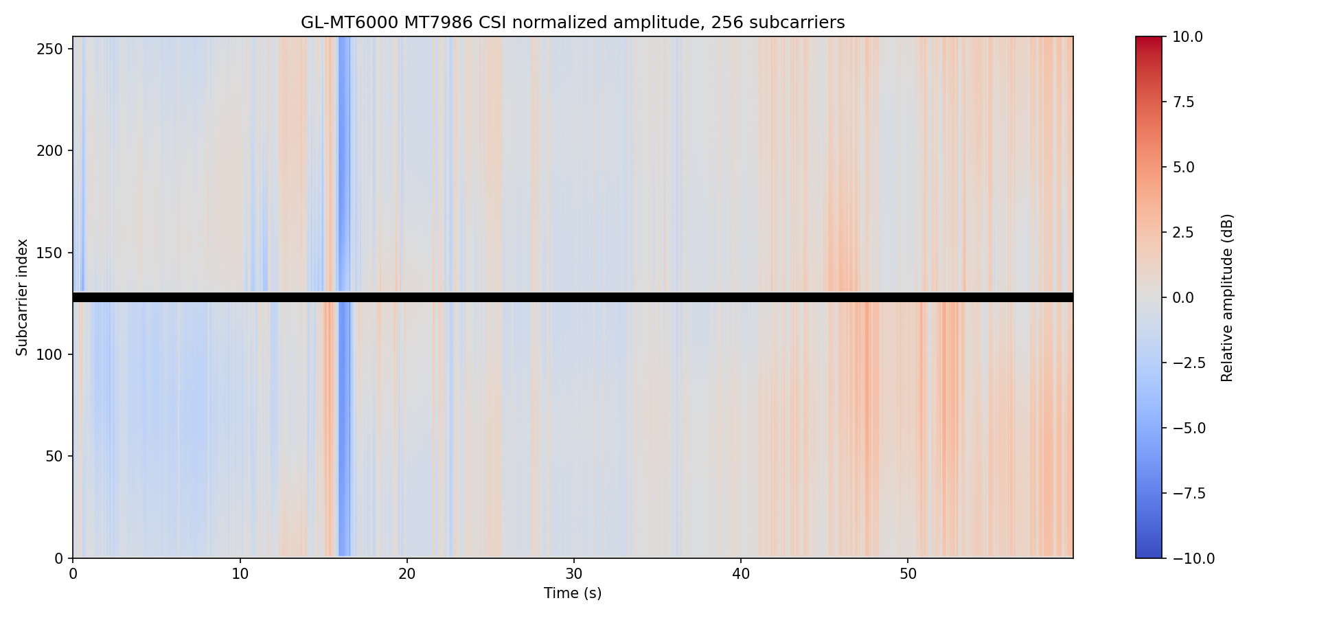
热图用于检查数据形状与时间稳定性,不用于证明某个动作分类器的准确率。
7. 验证清单
| 检查 | 10 分钟数据预期 |
|---|---|
| 外层记录 | 57,293 |
| bit15 完整测量组 | 7,609 |
| 链数分布 | 8 链 6,714 组;4 链 895 组;尾记录 1 |
| 简单选链后的矩阵 | 约 7,608 × 256 |
| 完整脚本剔除异常后的测量 | 7,583 |
| 时间跨度 | 约 599.92 秒 |
| 独立测量率 | 约 12.64–12.68 Hz |
| 整包 SHA-256 | 与 manifest 一致 |
如果这些值不一致,先检查:分片顺序、24/28 字节偏移、大小端、chain_info bit15、尾部不完整记录。
8. 内存与性能
| 数据 | 粗略内存 |
|---|---|
| 原始文件 | 约 58MB |
| 7,600 × 256 float64 幅度 | 约 15.6MB |
| 单链复数 CSI | 约 31MB |
| 8 条链全部复数 CSI | 约 250MB |
| 插值到 20Hz 的幅度矩阵 | 约 49MB |
长时间采集应逐条写入磁盘或按 session 分块处理,不要无限累积 Python 列表。处理前先记录
data_num、时间跨度、最大空档和链接强度,避免把数据质量问题误判成算法问题。
9. 常见坑
| 坑 | 表现 | 处理 |
|---|---|---|
| 把链记录当时间采样 | 采样率虚高、频谱混叠 | 按 bit15 分组,每个测量选一条链 |
| 直接平均原始相位 | 不同链相位偏移抵消 | 先按子载波/时间校正,或使用 ratio |
| 用序号代替时间戳 | 频谱假峰 | 按 file_ts 排序并重采样 |
| 把运动指标叫多普勒 | 视频里“有峰”但速度无意义 | 明确它是幅度变化,不是速度 |
| 用公网吞吐测试 Wi-Fi | 宽带波动混入结果 | 优先内网可控流量 |
| 只保存处理后的特征 | 无法复现解析错误 | 保留原始 bin、脚本版本与摘要 |
10. 可下载实现与下一步
- Router CSI Toolkit v0.1.3:
包含
analyze_csi_capture.py与采集工具; - 工具下载页 和 SHA-256;
- 分片校验与热图:数据集解析实战;
- 生命体征:呼吸/心率处理链路;
- 多平台解析:CSIKit [4]、csiread [5]、SenseFi 基准 [6]。
下一步不要急着上深度学习。先用真实数据确认矩阵形状、时间轴、空档、选链和运动基线,再建立可解释特征。
参考与数据来源
本文的每条外部结论都标注来源与证据等级(分级标准);标注 E 级的是本项目可复现的实测数据。
- E 级 · 本项目实测
本项目 10 分钟实测抓包(57,293 条 / 600.0 s,SHA-256 00373f83…95e2)
Router CSI Lab · 2026
okwujun.pw/zh/datasets/ · 核实: 分片重组逐字节校验通过(2026-10-11) · 本地原始母片 SHA-256 为 00373f83…95e2;公开下载的是去标识派生文件,SHA-256 为 527466ce…a440,两者不可混用。 - E 级 · 本项目实测
Router CSI Lab — GL-MT6000 (MT7986) Wi-Fi CSI dataset, 10 s sample + 10 min capture
Router CSI Lab · 2026
doi:10.5281/zenodo.23434789 · 核实: CC BY 4.0;SHA-256 已发布;Zenodo DOI 10.5281/zenodo.23434789 · 数据集已获 Zenodo DOI(10.5281/zenodo.23434789),可直接引用。 - E 级 · 本项目实测
Router CSI Toolkit — 采集/分析/守护脚本(MIT,公开仓库)
Router CSI Lab · 2026
github.com/jjjwu/router-csi-toolkit · 核实: GitHub API 于 2026-11-02 核实公开仓库、抓包质量预检、成功 CI 与 v0.1.3 Release;归档 SHA-256 为 59f144c0…adea7 · 公开版含无第三方依赖的抓包质量预检;网页端检查器使用同一容器定义和边界口径。 - C 级 · 官方资料
Gi-z/CSIKit — Python CSI parsing and visualisation
G. Zhang
github.com/Gi-z/CSIKit · 核实: GitHub API 2026-10-11 (stars 307, MIT, last push 2025-02-19) · 支持 Atheros / Intel / Nexmon / ESP32 / FeitCSI / PicoScenes 多种格式。 - C 级 · 官方资料
citysu/csiread — fast Cython CSI parser
S. Zhu
github.com/citysu/csiread · 核实: GitHub API 2026-10-11 (stars 142, MIT, last push 2024-10-12) - C 级 · 官方资料
xyanchen/WiFi-CSI-Sensing-Benchmark (SenseFi) — deep-learning benchmark
X. Chen, et al.
github.com/xyanchen/WiFi-CSI-Sensing-Benchmark · 核实: GitHub API 2026-10-11 (stars 638, MIT, last push 2023-11-06)