Do 256 CSI subcarriers mean 256 independent dimensions? A two-capture GL-MT6000 redundancy audit
By Wu Jun · Updated 2026-11-01 · Wi-Fi CSI, subcarrier redundancy, PCA, effective dimensionality, GL-MT6000, MT7986 · 7 min read
Result first: in this 10-minute GL-MT6000 amplitude capture, the 256 array positions are not 256 independent observation dimensions. On a correlation-matrix PCA of per-snapshot normalized amplitudes, 6 components explain 90% of variance, 9 explain 95% and 20 explain 99%. The participation-ratio effective rank is 4.568732, and the median adjacent-bin correlation is 0.900779. This is not a claim that the router contains six physical sensors; it is a statistical dimensionality result for these two captures and this preprocessing.
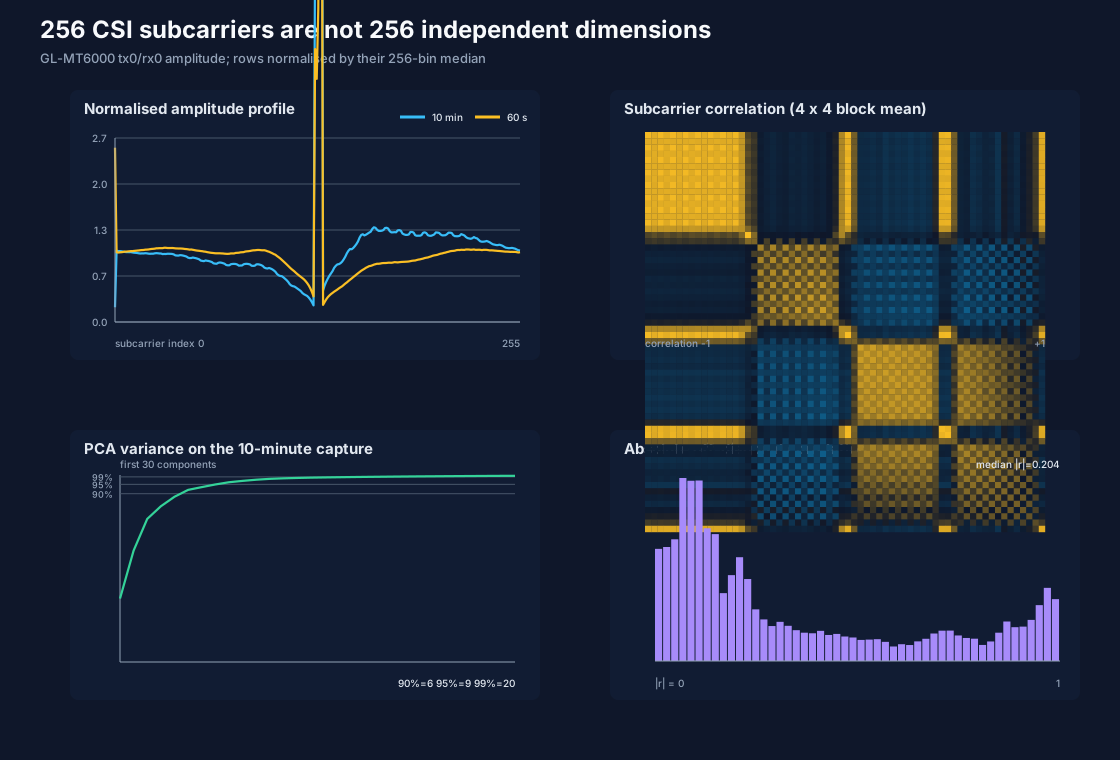
Figure 1: top left, normalized amplitude profiles for both captures; top right, a 4 x 4 block-averaged view of the 256 x 256 correlation matrix; bottom left, cumulative PCA variance for the 10-minute capture; bottom right, the absolute off-diagonal correlation distribution. The public script generates the figure.
1. Results
Both captures select tx0/rx0 only. The analysis never falls back to another chain and never
treats multiple tx/rx records as additional time samples [1].
| Metric | 10-minute capture | 60-second capture |
|---|---|---|
| Outer records | 57,293 | 2,777 |
| Closed bit-15 groups | 7,609 | 347 |
Complete 256-bin tx0/rx0 rows |
7,608 | 347 |
| Incomplete fixed-chain groups | 1 | 0 |
| Components for 90% cumulative variance | 6 | not used for dimension selection |
| Components for 95% cumulative variance | 9 | not used for dimension selection |
| Components for 99% cumulative variance | 20 | not used for dimension selection |
| Participation-ratio effective rank | 4.568732 | not used for dimension selection |
| First-component variance | 33.933% | not used for dimension selection |
| First 10-component cumulative variance | 96.858% | not used for dimension selection |
| Median absolute off-diagonal correlation | 0.204452 | not used for dimension selection |
| Median adjacent-bin correlation | 0.900779 | not used for dimension selection |
Pairs with abs(r) >= 0.75 |
17.451% | not used for dimension selection |
Pairs with abs(r) >= 0.90 |
10.064% | not used for dimension selection |
The 10-minute capture supplies the PCA dimensionality result. The 60-second capture is used only to ask whether a similar structure appears again; it does not select the number of components. This avoids leaking the comparison session into model selection.
2. Why 256 columns are not 256 degrees of freedom
A CSI frame is often flattened into a 256-dimensional vector. A later model may implicitly assume that each column is independent, or apply ordinary table-style feature selection. But nearby frequency positions share the transmitter, receiver, multipath, automatic gain and capture layout. A column count is not a measure of independent information [2] [3].
The distinction affects:
- parameter count and collinearity in linear models;
- the preferences of tree models and neural networks for redundant inputs;
- whether train/test splits represent genuinely independent evidence;
- whether a 256-column visualisation is mistaken for 256 physical sensors;
- compression, storage, inference latency and edge-device budgets.
PCA does not establish the physical cause of a correlation. It describes how variance is distributed in the current matrix [4]. This article therefore reports correlation structure and statistical dimensionality, not “the hardware has only a few subcarriers”.
3. Data selection and preprocessing
The pipeline is:
- walk the outer
<float64 ts><uint16 len><payload>container; - close a measurement group on
chain_infobit 15; - select
tx0/rx0; count missing or duplicate fixed-chain groups and skip them rather than silently substituting another chain; - accept only complete 256-complex-pair records with non-zero I/Q;
- divide each 256-bin amplitude vector by its own median to remove the first-order shared gain;
- centre and scale each bin over time to unit standard deviation;
- eigendecompose the resulting 256 x 256 Pearson correlation matrix;
- define the dimension threshold as the first component count reaching 90%, 95% or 99% cumulative variance;
- also report a participation-ratio effective rank:
effective_rank = (sum(eigenvalues)^2) / sum(eigenvalues^2)
Of the 7,609 closed groups in the 10-minute data, 7,608 are complete 256-bin fixed-chain rows;
one group is not a complete fixed-chain sample. All 347 closed groups in the 60-second capture
are usable. Input SHA-256 values are
527466ceb8b5f835e55ff348f02808736b947db39e7baac1f34e375de146a440 and
41c35d9d23e5c03ddd34ae97617e772fecdb55e8545156181828b060605a87a6.
4. The correlation structure is layered, not uniformly high
Across the 32,640 off-diagonal bin pairs, the median absolute correlation is only 0.204452. Considered alone, that number can create the false impression that the bins are mostly independent. The upper tail is different:
- p95 of
abs(r)is 0.960370; - 17.451% of pairs reach
abs(r) >= 0.75; - 10.064% reach
abs(r) >= 0.90; - the median adjacent-bin correlation is 0.900779, with a mean absolute adjacent correlation of 0.856893.
A better description is therefore: nearby positions form strong local structures, many distant pairs are weakly correlated, and the matrix is not one uniform 256 x 256 block. A low median and a low PCA dimension are not contradictory; a small number of strong directions dominate the eigenspectrum.
The matrix cannot assign physical frequencies to array indices. Mapping indices to OFDM subcarriers, pilots, guard bands or resource units requires driver and firmware evidence that this experiment does not provide.
5. The 6 / 9 / 20 dimension thresholds
The leading eigenvalues of the 10-minute correlation matrix are:
| Component | Variance share | Cumulative |
|---|---|---|
| 1 | 33.933% | 33.933% |
| 2 | 25.669% | 59.602% |
| 3 | 16.927% | 76.528% |
| 4 | 6.754% | 83.283% |
| 5 | 5.088% | 88.370% |
| 6 | 3.670% | 92.041% |
| 7 | 1.477% | 93.518% |
| 8 | 1.415% | 94.934% |
| 9 | 1.194% | 96.127% |
| 10 | 0.730% | 96.858% |
Therefore:
- preserving 90% variance needs 6 dimensions instead of 256;
- preserving 95% needs 9;
- preserving 99% needs 20;
- the participation ratio reports 4.568732 because it gives more weight to the largest eigenvalues; it is not the same criterion as the 90% threshold;
- every reduction discards tail variance, and whether that is acceptable must be decided by a downstream task and independent validation.
It is also incorrect to call these six components “six physical paths”. PCA only provides a rotation ordered by squared variance under the chosen representation; it does not guarantee physical interpretability or cross-device alignment.
6. Does the 60-second capture reproduce the structure?
After normalizing each capture by its own 256-bin row median, the per-bin median amplitude profiles have:
- Pearson correlation 0.954781;
- temporal-CV profile correlation 0.984305;
- mean L1 distance between median profiles 0.267042.
The relative bin structure is highly similar across these captures. Absolute gain is not the same, so this cannot be described as unchanged absolute amplitude or link budget.
Per-bin temporal variability is also highly uneven:
| Metric | 10-minute | 60-second |
|---|---|---|
| Minimum CV | 0.087431 | 0.056579 |
| CV p25 | 0.173107 | 0.102854 |
| Median CV | 0.248880 | 0.135704 |
| CV p75 | 9.274449 | 7.475848 |
| CV p95 | 10.816894 | 7.849462 |
| Maximum CV | 12.641809 | 8.561378 |
Share of bins with CV > 1 |
37.891% | 36.328% |
The distribution is strongly skewed. A high CV is not automatically bad data and does not prove greater sensing sensitivity. Local nulls, gain changes, multipath and capture layout can all contribute. The analysis publishes the per-bin values and does not delete them by a CV rule.
In the 10-minute capture, 127 bins contain at least one zero amplitude, with about 400 zero-bin observations in total; the largest per-bin zero fraction is about 0.131%. The 60-second capture has 47 such bins and about 55 observations, with a maximum fraction of about 0.576%. The number is small but non-zero, so a parser must handle it rather than divide by zero or fill silently.
7. Consequences for modelling and experiment design
A more defensible practice is:
- describe the 256-dimensional input as a redundant raw representation, not 256 independent sensors;
- report correlations and effective dimensionality within each session;
- if PCA or another reduction is used, choose its dimension on a training session only;
- evaluate on an unseen session or room rather than declaring generalisation from a random split of one capture;
- compare the raw 256-dimensional input with lower-dimensional representations across linear, tree and neural models instead of assuming reduction is automatically better;
- publish bin identity, preprocessing and the eigenvalue spectrum rather than only an accuracy number.
“Six components explain 90%” does not mean every task needs only six features. A task may depend on weak tail signals, specific pilots or local nulls. The correct question is how much tail variance can be discarded for this task and this independent test protocol.
8. Reproduce
Download the public 10-minute capture and 60-second demo source, then run:
python3 analyze_csi_subcarrier_redundancy.py \
  csi_udp_20261010_10m.anon.bin \
  csi_demo_60s_anonymized.bin \
  --out-dir csi-subcarrier-redundancy \
  --img csi-subcarrier-redundancy.svg
The script requires Python 3.9+ and NumPy only. Public files:
- Analysis script
- Machine-readable summary
- 256-row subcarrier metrics CSV
- 256-eigenvalue CSV
- Reproduction notes
- SHA-256 checksums
See the GL-MT6000 Wi-Fi CSI dataset for the source captures, the chain-health audit for missing-chain behaviour, and the timestamp-gap spectral analysis for the sampling-time consequences.
9. Evidence boundaries
This is a first-party, reproducible analysis (grade E) [5], with the PCA method context taken from a peer-reviewed review [4]. It does not prove:
- that an array index corresponds to a specific OFDM subcarrier, pilot or physical antenna;
- a unique physical cause for the observed correlations;
- that another GL-MT6000, firmware, room or client will produce exactly 4.568732 effective dimensions;
- that these components can be used for respiration, fall, occupancy, identity or medical decisions;
- that a lower-dimensional representation improves every classifier.
Both captures lack an empty-room baseline, known actions, subject position and human-event ground truth. The experiment supports amplitude-redundancy auditing, dimension reporting and stricter experimental design only.
10. Acceptance checklist
- Fix the chain and count missing-chain groups instead of silently substituting one;
- report closed groups and usable rows for each capture;
- state the per-snapshot normalization and per-bin standardization;
- publish both the correlation distribution and eigenvalue spectrum;
- test whether the structure reappears in an independent session;
- choose dimensions on the training session only;
- publish the script, JSON, per-bin CSV, eigenvalue CSV, figure and SHA-256;
- do not translate statistical dimensions into a physical sensor count.
References and data sources
Every external claim carries a source and an evidence grade (grading scheme). Grade E marks first-party, reproducible measurements from this project.
- Grade E · first-party measurement
This project's 10-minute raw capture (57,293 records / 600.0 s, SHA-256 00373f83…95e2)
Router CSI Lab · 2026
okwujun.pw/en/datasets/ · verified: Reassembled chunks verified byte-identical (2026-10-11) · The local raw master has SHA-256 00373f83…95e2; the public de-identified derivative has SHA-256 527466ce…a440. They must not be confused. - Grade A · standard/review
WiFi Sensing with Channel State Information: A Survey
W. Ma, W. Zhou, X. Wang · ACM Computing Surveys · 2019
doi:10.1145/3310194 · citations 857 · verified: CrossRef API, 2026-10-11 · The field's most-cited CSI sensing survey (857 citations, verified via CrossRef). - Grade B · peer-reviewed
Tool release: gathering 802.11n traces with channel state information
D. Halperin, W. Hu, A. Sheth, D. Wetherall · ACM SIGCOMM Computer Communication Review · 2011
doi:10.1145/1925861.1925870 · citations 1713 · verified: CrossRef API, 2026-10-11 · The formal paper for the Intel 5300 CSI Tool (1713 citations) — the widely reproduced starting point for CSI capture. - Grade B · peer-reviewed
Principal component analysis: a review and recent developments
I. T. Jolliffe, J. Cadima · Philosophical Transactions of the Royal Society A · 2016
doi:10.1098/rsta.2015.0202 · citations 7798 · verified: CrossRef API, 2026-11-01 · A peer-reviewed PCA review covering explained variance, dimensionality reduction and interpretation limits. This article uses it for the method definition, not as causal evidence for the observed correlation. - Grade E · first-party measurement
CSI subcarrier redundancy and effective-dimensionality audit (script, metrics, PCA spectrum)
Router CSI Lab · 2026
okwujun.pw/en/csi-subcarrier-redundancy/ · verified: Rerun from the public 10-minute and 60-second captures with input SHA-256 527466ce…a440 and 41c35d9d…87a6; script, JSON, CSVs and figure are published together (2026-11-01) · This establishes correlation structure and effective dimensionality in these two amplitude captures only. It does not map array indices to physical frequencies or provide human ground truth. - Grade E · first-party measurement
Router CSI Toolkit — capture/analysis/watchdog scripts (MIT, public repository)
Router CSI Lab · 2026
github.com/jjjwu/router-csi-toolkit · verified: GitHub API verified the public repository, capture-quality preflight, successful CI and the v0.1.3 release on 2026-11-02; the archive SHA-256 is 59f144c0…adea7 · The public repository includes a dependency-free capture preflight; the browser checker uses the same container definition and evidence boundaries.