The spectral cost of CSI timestamp gaps: a controlled test on real sampling times
By Wu Jun · Updated 2026-10-30 · Wi-Fi CSI, timestamps, missing data, spectrum, Lomb-Scargle, reproducibility · 6 min read
Result first: the 10-minute capture has an average usable-group rate of about 12.68 groups/s, but it is not a uniform 12.68 Hz clock. After linear interpolation to a 10 Hz grid, 1,823 of 6,000 points (30.383%) lie inside original intervals longer than 0.5 s. For a known 0.25 Hz sinusoid placed on the real timestamps, interpolation has an RMS error of 0.099658 (14.094% of the signal RMS), while a least-squares fit on the original timestamps still returns 0.250 Hz. This is not a breathing or human experiment, but it is enough to reject the practice of interpolating first and treating the resulting peak as a physiological fact.
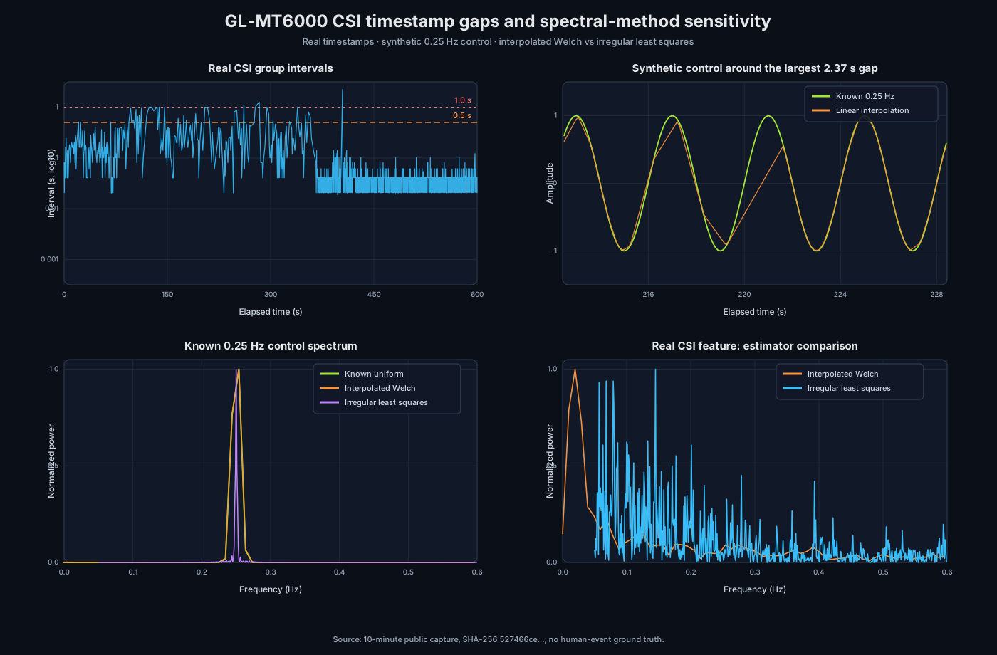
Four panels show the original group intervals, a known 0.25 Hz control around the largest 2.37 s gap, the control spectrum, and two estimators on the real CSI amplitude feature. The public script generates the figure from the same input.
1. Why an average rate is not a timebase
The public capture contains 57,293 outer chain records. Grouping on chain_info bit 15 produces 7,609
measurement groups; after excluding one 64-subcarrier transition group, 7,608 usable 256-subcarrier
groups remain [1]. The average group rate is:
7608 / 599.924 s = 12.6817 groups/s
The average is not the sampling clock. The observed interval median is about 41.02 ms, p95 is 321.84 ms, p99 is 945.69 ms, and the maximum is 2.373 s. There are 224 intervals longer than 0.5 s and 57 longer than 1 s. A running collector does not imply that every intended timestamp left a CSI snapshot.
An algorithm that reads only “12.68 Hz” can treat a timeline with long gaps as a regular sequence. FFT, STFT, band-pass filtering and peak detection then inherit the error. The data layout and source capture are documented on the dataset page, and the timing audit is reproducible from [2].
2. What the experiment compares
For every usable group this experiment selects one representative chain: prefer tx0/rx0; otherwise
use the valid chain with the largest mean amplitude. The feature is the mean amplitude across the
selected chain's 256 subcarriers. All 7,608 groups selected tx0/rx0, so multiple receive chains are
never counted as independent time samples.
Three paths are compared:
- Uniform grid + interpolated Welch: map the original timestamps to a 10 Hz grid with
np.interp, then use a 1024-sample Hann-window Welch estimate; - Direct fit on original timestamps: fit sine/cosine terms from 0.05 to 0.60 Hz at 0.001 Hz spacing. This is a Lomb-Scargle-family least-squares estimator [3] [4];
- Known-signal control: place a unit-amplitude 0.10-0.50 Hz sinusoid on the real timestamps and compare the interpolated values with the exact values.
The third path matters. The real CSI has no respiration or motion ground truth. A known sinusoid does: it separates “what is in the signal” from “what the preprocessing created or distorted”.
3. How much of the 10 Hz grid is interpolated?
The 10 Hz grid contains 6,000 points over 599.924 s and is suitable for inspecting 0.05-4 Hz components (Nyquist 5 Hz). Of those points, 1,823 lie inside original intervals longer than 0.5 s, which is 30.383% of the grid. This does not mean 30% of the source was lost; it means those grid values have no original snapshot at exactly that time and must be synthesized from neighbours.
The strict continuous-window alternatives are also constrained:
| Segment rule | Segments of at least 20 s | Covered time |
|---|---|---|
| No interval over 0.5 s | 2 | 231.90 s |
| No interval over 1.0 s | 6 | 391.45 s |
Thus “run Welch only on continuous windows” is not free: tighter thresholds discard more time. The correct response is not hidden interpolation; it is to report gaps, available windows, loss fraction and the frequency range where the result is defensible.
4. Known 0.25 Hz control
0.25 Hz is near a commonly discussed respiration band, but here it is only a controlled mathematical signal, not a breathing recording.
| Metric | Result |
|---|---|
| True frequency | 0.250 Hz |
| Exact 10 Hz-grid Welch peak | 0.253906 Hz (frequency-bin limit 0.009766 Hz) |
| Interpolated Welch peak | 0.253906 Hz |
| Original-timestamp least-squares peak | 0.250 Hz |
| Interpolation RMS error | 0.099658 |
| Maximum absolute interpolation error | 1.09835 |
| Relative signal-RMS error | 14.094% |
| 0.10-0.50 Hz band-power retained | 88.64% |
The control shows why “the peak frequency did not move much” is not enough. Interpolation can preserve the approximate peak location while changing the waveform, amplitude and local time structure. That matters for comparing depth, harmonics, event onset or recovery. The estimated band power is about 11.36% lower than the exact control even when the peak is on a nearby bin.
5. Higher frequencies pay a larger relative cost
Changing the known sinusoid on the same real timeline gives:
| True frequency | Relative RMS error | Interpolated Welch peak | Original-timestamp peak |
|---|---|---|---|
| 0.10 Hz | 2.31% | 0.097656 Hz | 0.100 Hz |
| 0.15 Hz | 4.72% | 0.146484 Hz | 0.150 Hz |
| 0.20 Hz | 9.80% | 0.195312 Hz | 0.200 Hz |
| 0.25 Hz | 14.09% | 0.253906 Hz | 0.250 Hz |
| 0.30 Hz | 18.40% | 0.302734 Hz | 0.300 Hz |
| 0.40 Hz | 27.85% | 0.400391 Hz | 0.400 Hz |
| 0.50 Hz | 38.16% | 0.498047 Hz | 0.500 Hz |
Frequency is not the only variable: gap position, phase and relative gap duration also matter. The
table still rules out casually extrapolating a 0.25 Hz result to every band. The complete sweep is in
frequency_sweep.csv.
6. The real CSI estimators disagree
On the same real amplitude feature, the interpolated Welch estimate has its highest point at 0.068359 Hz in the 0.05-0.60 Hz search range. The least-squares fit on the original timestamps peaks at 0.145 Hz. The difference is 0.076641 Hz.
This does not prove that 0.145 Hz is a person and it does not prove that 0.068 Hz is an artifact. It does prove a more basic fact: without time truth, event labels or a reference sensor, the preprocessing choice alone can change the reported dominant frequency. A claim such as “breathing at 0.145 Hz” cannot be audited if the interpolation rule is hidden.
7. Practical rules
Preserve time
Keep the outer timestamp, payload timestamp, group boundary and chain-selection rule. Do not save only an average sampling rate; it cannot reconstruct gaps or irregular observations.
Audit before FFT
Report at least:
- group-interval median, p95, p99 and maximum;
- counts of gaps over 0.5, 1 and 2 seconds;
- uniform-grid point count and the fraction inside long gaps;
- interpolation boundary and extrapolation policy;
- continuous-window length and coverage used by the final spectrum.
Use an irregular method or an explicit mask
For respiration, slow motion and long events, prefer a direct irregular-time periodogram or Welch computed on short continuous segments with coverage reported. Either way, run a frequency/gap/estimator sensitivity check. Do not turn one algorithm's peak into a physiological conclusion.
Do not fill fall or fast-event structure with interpolation
Fall analysis depends on event onset, recovery and context. Interpolation smooths boundaries and can change short-time energy and recovery features. The existing 12.64 groups/s capture rate also does not support full gait micro-Doppler; see fall detection and CSI radar limits.
8. Reproduce
Download the public 10-minute capture and run:
python3 analyze_csi_gap_spectrum.py csi-10m.anon.bin \
  --summary summary.json \
  --csv frequency_sweep.csv \
  --img csi-gap-spectrum.svg
The script needs Python 3.9+ and NumPy only; it does not require Matplotlib or SciPy. Public files:
The public de-identified input capture has SHA-256
527466ceb8b5f835e55ff348f02808736b947db39e7baac1f34e375de146a440.
9. Evidence boundaries
This is a first-party, reproducible analysis (grade E) [5], with sampling-method background from peer-reviewed work [3] [4] [6]. It does not include:
- breathing or human ground truth, subject position, motion labels or fall labels;
- generalisation across rooms, clients, traffic profiles or firmware versions;
- a complete noise-model and significance validation of the irregular estimator;
- evidence that a 10 Hz interpolation can recover all CSI information.
10. Acceptance checklist
- Report records, groups, interval distribution and maximum gap;
- State the selected chain and confirm bit-15 grouping;
- State the uniform rate and interpolation method;
- Report the fraction of grid points inside long gaps;
- Compare against an irregular-time or continuous-segment method;
- Test interpolation with a known sinusoid control;
- Keep “observed peak” separate from “human ground truth”;
- Publish script, summary, CSV, figure and SHA-256.
References and data sources
Every external claim carries a source and an evidence grade (grading scheme). Grade E marks first-party, reproducible measurements from this project.
- Grade E · first-party measurement
This project's 10-minute raw capture (57,293 records / 600.0 s, SHA-256 00373f83…95e2)
Router CSI Lab · 2026
okwujun.pw/en/datasets/ · verified: Reassembled chunks verified byte-identical (2026-10-11) · The local raw master has SHA-256 00373f83…95e2; the public de-identified derivative has SHA-256 527466ce…a440. They must not be confused. - Grade E · first-party measurement
Router CSI Lab — GL-MT6000 (MT7986) Wi-Fi CSI dataset, 10 s sample + 10 min capture
Router CSI Lab · 2026
doi:10.5281/zenodo.23434789 · verified: CC BY 4.0; SHA-256 published; Zenodo DOI 10.5281/zenodo.23434789 · The dataset has a Zenodo DOI (10.5281/zenodo.23434789) and can be cited directly. - Grade B · peer-reviewed
Least-squares frequency analysis of unequally spaced data
N. R. Lomb · Astrophysics and Space Science · 1976
doi:10.1007/BF00648343 · citations 5106 · verified: CrossRef API, 2026-10-30 · A classical least-squares frequency-analysis method for unevenly spaced time series. This article cites it only at the method level and does not assume CSI satisfies its noise model. - Grade B · peer-reviewed
Studies in astronomical time series analysis. II. Statistical aspects of spectral analysis of unevenly spaced data
J. D. Scargle · The Astrophysical Journal · 1982
doi:10.1086/160554 · citations 6463 · verified: CrossRef API, 2026-10-30 · The statistical basis of the Lomb-Scargle periodogram and why the original observation times matter instead of inventing a uniform grid first. - Grade E · first-party measurement
CSI timestamp-gap spectral sensitivity analysis (script, summary, frequency sweep)
Router CSI Lab · 2026
okwujun.pw/en/csi-timestamp-gaps-spectrum/ · verified: Rerun from the public 10-minute capture with input SHA-256 527466ce…a440; script, JSON, CSV and figure are published together (2026-10-30) · This establishes method sensitivity on this sampling timeline only; it provides no respiration, fall or human ground truth. - Grade B · peer-reviewed
Understanding the Lomb–Scargle Periodogram
J. T. VanderPlas · The Astrophysical Journal Supplement Series · 2018
doi:10.3847/1538-4365/aab766 · citations 1182 · verified: CrossRef API, 2026-10-30 · A practical review of the Lomb-Scargle periodogram, emphasising sampling, windowing, noise and significance assumptions. It informs the stated limits here.